

What are the CMAPF routines?
The CMAPF routines are libraries of tools – functions and subroutines that allow meteorological model programs to be independent of the choice of map projection on which their model is based. Most models are based on a rectangular lattice of mesh points drawn on some specific map, the choice of which depends on a number of considerations, including the size and location of the region to be modeled. The geometry of the map introduces subtle changes in the equations describing the physics of the model, whose terms are provided by calls to these subroutines.
When a model requires input data from another source, which was gridded on some other mesh drawn on some other map projection, the CMAPF routines can accomplish the translation from one to the other, since they can work with several projections concurrently.
What Map Projections do the CMAPF routines deal with?
There are two versions of the CMAPF routines, version 1.0 and 2.0. Version 1.0 covers the standard conformal map projections centered at the North and South Pole, namely the Polar Stereographic, the Mercator, and the Lambert Conformal projections.
Version 2.0 covers the same set of conformal routines, but instead of being restricted to centering on the poles, they may be centered on an equatorial point (Transverse Mercator) or on any other point (Oblique Stereographic).
CMAPF Links and Installation information
FAQ
CMAPF FAQ is below
EMAPF
Installing The EMAPF Functions
Using the EMAPF Functions (Fortran)
CMAPF
Using The Cmapf Routines (FORTRAN)
DMAPF
Using The Dmapf Routines (FORTRAN)
Download Libraries
CMAPF libraries: Version 1.0 (13.6 Kb, gz)
DMAPF libraries: Version 2.0 (21.4 Kb, gz)
EMAPF libraries: Unknown version (207 Kb, gz)
CMAPF FAQ
In what language can I access the CMAPF routines?
The CMAPF function libraries were written in FORTRAN and in C. Both versions are essentially the same, except for minor variations to accommodate the differences in language.
Where can I find out more about the CMAPF functions?
Version 1.0 is described more fully in an article, Conformal Map Transformations for Meteorological Modelers, by Albion D. Taylor, published in the February, 1997 issue of Computers and Geosciences (v23, no 1): https://doi.org/10.1016/S0098-3004(96)00062-3. An FAQ is below.
How do I use the CMAPF libraries?
Instructions for using the routines are summarized in the C-version and in the FORTRAN-version.
How do I obtain the CMAPF libraries?
Version 1.0 (13.6 Kb, gz) is available for download here.
How do I obtain the DMAPF libraries?
Version 2.0 (21.4 Kb, gz), is now available here. This version (also known as the Dmapf routines) adds Oblique and Transverse projections to the normal projections to the normal projections covered by version 1.0. That is, projections can be oriented around any diameter of the Earth, rather than just the Polar axis, which can be convenient for smaller scale local grids. Instructions on the use of the Dmapf routines are available for both the C-language and the FORTRAN language.
In addition, several display utility routines using Dmapf can be installed on 32-bit Windows platforms (Windows 95 and later).
How do I obtain the EMAPF libraries?
The EMAPF library (207 Kb, gz), is now available here. The Emapf routines are an extension of the CMAPF functions to accommodate Ellipsoidal Geoids. Instructions on the use of the Emapf routines are available for both the C-language and the FORTRAN language. EMAPF installation instructions are also available.
CMAPF FAQ:
- Where do I find more about the CMAPF functions?
- In what language can I access the CMAPF routines?
- What units are the x-y coordinates in?
- Why is the initialization of the projections split into two stages?
- What is the meaning of REFLAT and REFLON in STLMBR? What values do I use?
- How do I relate the parameters in CMAPF to the Grid Descriptions in GRIB?
- Why do we need the EQVLAT function? Can’t we just use the midpoint of the reference latitudes REFLT1 and REFLT2 i.e.
.5*(REFLT1+REFLT2)as the tangent latitude for the cone? - Which two points do I use in the STCM2P initialization? The diagonally opposite corners (lower left and upper right)?
- Explain the parameters in the STCM1P routine. Why do you call it one-point, when you use latitude-longitude coordinates for two points?
- How big is the Earth? Which radius should I use in compiling and using your programs? What difference would using the wrong radius make?
- The legend on Lambert Conformal Projections usually have two reference latitudes. The projection is drawn on a cone that passes through these two latitude circles, right? (WRONG!!)
- The Mercator projection is done by drawing rays from the Earth’s center through points on the Earth’s Surface to a cylinder tangent to the Earth at the Equator, right? (WRONG!!)
- The Lambert Conformal Projection is also known as the Albers equal-area Projection, right? (WRONG!!)
- Is it unreasonable to make a tangent specification with a secant specification whose latitudes are the same?
- So why do printed and published Lambert Projection maps invariably use two reference latitudes?
- Are you sure the Lambert cone doesn’t pass through the Earth at the reference latitudes?
Answers:
- Where do I find more about the CMAPF functions?
CMAPF is described more fully in an article, Conformal Map Transformations for Meteorological Modelers, by Albion D. Taylor, published in the February, 1997 issue of Computers and Geosciences (v23, no 1) It is also available here and source code in C and FORTRAN may be downloaded here. Instructions on the individual functions and subroutines are available here for FORTRAN and here for C. - In what language can I access the CMAPF routines?
Two CMAPF function libraries were written, one in FORTRAN and one in C. Both versions are essentially the same, except for minor variations to accommodate the differences in language. - What units are the x-y coordinates in?
The original point of the CMAPF routines was to convert the indices I,J of meteorological grid points to latitude-longitude coordinates and back again. Because arbitrary latitude-longitude coordinates, more often than not, will appear in the interior of a grid cell, the I,J indices must be floating point numbers rather than integers, and hence by convention referred to as X,Y rather than I,J. By either reference, the X,Y coordinates are non-dimensional. I.e., units are grid-cells. If your purpose is something other than meteorological grids, such as drawing maps on paper, then X,Y can be in whatever units are appropriate, such as inches of paper. Such units would automatically be allowed for when defining scales through STCM1P or STCM2P, since the numeric values used for X,Y in those routines will be expressed in your intended units. - Why is the initialization of the projections split into two stages?
The first stage, the STLMBR routine, specifies the projection’s shape only. It defines whether we are dealing with a Lambert Conformal projection on a cone, a Mercator projection on a cylinder, or a Polar Stereographic projection on a plane. This is analogous to selecting a map on which to lay out your grid. The second stage specifies the projection’s scale in grid units, as well as its origin and orientation, using either STCM1P or STCM2P. This is analogous to laying out your grid on the selected map. The scale, orientation and origin of a grid can be changed any number of times without altering the shape of the projection, but any change in the shape of the projection will disrupt the scale and orientation, which will need to be respecified. Analogously, you can lay out many rectangular grids on a given map, but if the map is changed, the grid will no longer be rectangular. - What is the meaning of REFLAT and REFLON in STLMBR? What values do I use?
REFLAT is the angle at which the cone of a Lambert Conformal projection is tangent to the Earth. It may be a very narrow, long cone tangent to a circle of latitude at a low latitude, or a very fat, almost planar cone tangent at a high latitude, or a moderate shape cone tangent at a mid latitude. The shapes of features on the Earth will suffer the least distortion near this latitude. If REFLAT is 90., the cone becomes a plane at the North pole; i.e. a Polar Stereographic projection, and this is how a Polar Stereographic projection is specified. If REFLAT is 0., the cone becomes a cylinder tangent at the equator, and this is how a Mercator projection is specified. REFLON is the longitude furthest from the cut. Any Lambert conformal projection (i.e. on a cone) or Mercator projection (i.e. on a cylinder) must have the cone or cylinder cut along a meridian before it can be unrolled onto a plane. We want our grids to be well clear of this cut; if the cut runs through our grid, it can cause major geometrical problems. By selecting REFLON to pass through our grid, we get 180 degrees of longitude in either direction as room to work with. The Polar Stereographic projection (on the plane, REFLAT=90.) has no cut, so for this case, REFLON can be specified arbitrarily. - How do I relate the parameters in CMAPF to the Grid Descriptions in GRIB?
GRIB (GRIdded Binary), is a general purpose, bit-oriented data exchange format, designated FM 92-VIII Ext. GRIB by the World Meteorological Organization (WMO) Commission for Basic Systems (CBS). It is documented in Dey, Clifford H., “NATIONAL CENTERS FOR ENVIRONMENTAL PREDICTION OFFICE NOTE 388”, Mar, 1998 (unpublished) available here in WordPerfect and Adobe Acrobat (.pdf) formats. Individual grids are listed in section 1 of that document, in table B, while definitions of terms are in section 2, in Table D. The Grid Descriptions of interest to us are Polar Stereographic (section 2, page 9), Lambert Conformal (Section 2, Page 10), and Mercator (Section 2, Page 11). We consider each separately.A. Polar Stereographic Grids. The CMAPF call to initialize the shape of any Polar Stereographic projection isCALL STLMBR(PARMAP, 90.,0.)if tangent at the North pole, orCALL STLMBR(PARMAP, -90.,0.)if tangent at the South Pole. GRIB’s GDS octet 27 determines whether to use the North or South Pole. Data in GRIB’s Polar Stereographic section is in a form best suited to one-point initialization (STCM1P). Using the terminology there, we would initialize through the callCALL STCM1P(PARMAP, 1.,1., La1/1000.,Lo1/1000.,60.,Lov/1000., Dx/1000.,0.)The divisions by 1000. are due to the fact that units in GRIB are millidegrees of latitude and longitude, and grid sizes in meters, while CMAPF expects degrees and kilometers. The call means that grid point 1,1 is mapped into the point at latitude/longitude given by La1,Lo1, the gridsize is referred to the 60 latitude (according to note 2 in the GRIB document (the -60 latitude if the South polar projection is used), and the Lov meridian is vertical (ORIENT=0.)B. Lambert Conformal Grids. The CMAPF call to initialize the shape of a Lambert Conformal Projection is
CALL STLMBR(PARMAP, EQVLAT(Latin1/1000., Latin2/1000.), Lov/1000.)
The EQVLAT function will return a tangent latitude that ensures the scale at latitude Latin1 is the same as that at Latin2, i.e. the projection defined by the two reference latitudes. If Latin1=Latin2, EQVLAT will return their common value. REFLON can be set either to Lov or Lo1, whichever ensures the cut is well away from the grid areas.
Data in GRIB’s Polar Stereographic section is in a form best suited to one-point initialization (STCM1P). Using the terminology there, we would initialize through the call
CALL STCM1P(PARMAP, 1.,1., La1/1000.,Lo1/1000., Latin1/1000.,Lov/1000., Dx/1000.,0.)
Either Latin1 or Latin2 can be used for the latitude at which the gridsize is Dx/1000., because the use of EQVLAT in the call to STLMBR has guaranteed that the scale is the same at Latin1 as it is at Latin2.
CALL STLMBR(PARMAP, 0., (Lo1 + Lo2)/2000.)
Note: the value of REFLAT in a Mercator projection is always zero, has no relation to the “Latin” value specified in GRIB, and must not be confused with it. Specifying REFLON to be the midpoint of the grid will allow as much space as possible between the grid and the cut.
From the information in GRIB, we may choose whether to use one-point or two-point specification.
We may use the information on one point, gridsize and orientation to specify
CALL STCM1P(PARMAP, 1.,1., La1/1000.,Lo1/1000., Latin/1000.,0., Di/1000.,0.)
since any meridian, including the 0° meridian in the above code example, can be the reference meridian set to vertical with ORIENT=0., and Di is the grid size at reference latitude Latin.
On the other hand, we may use the information on two points to specify
CALL STCM2P(PARMAP, 1.,1., La1/1000.,Lo1/1000., Ni*1.,Nj*1., La2/1000.,Lo2/1000.)
to scale and orient the map.
If we do it both ways, and compare the results, we have a check on the internal consistency of the grids.
- Why do we need the EQVLAT function? Can’t we just use the midpoint of the reference latitudes REFLT1 and REFLT2 (i.e.
.5*(REFLT1+REFLT2)) as the tangent latitude for the cone?
The EQVLAT function returns a value for tangent latitude that is generally somewhat different from the midpoint latitude, and further from the equator. EQVLAT is provided to guarantee that the scale of the map is the same at latitude REFLT1 as it is at REFLT2, and therefore as nearly uniform and undistorted as geometrically possible in the latitude range between. The midpoint latitude does not guarantee equal scales at the two reference latitudes. Indeed, the gridsize would be smaller at the reference latitude closer to the pole, so there would be an overall scale gradient with consequent distortion. It is sometimes pointed out that the midpoint latitude produces a projection cone which, properly aligned on the Earth’s axis, will pass through both the two given circles of latitude on a spherical Earth. While this is true, it is an academic consideration to the practical map user, who is more concerned with scale gradient distortion of his map. - Which two points do I use in the STCM2P initialization? The diagonally opposite corners (lower left and upper right)?
Not necessarily. Any two different points, for which you know both the x,y and the latitude,longitude coordinates will do. To reduce the effect of measurement errors, it is a good idea to keep them as far from each other as possible, and diagonally opposite corners does just that. However, if you are laying out a rectangular grid on a Mercator projection, and you want to make sure the grid is aligned North-South and East-West, it is easier to use the two lower corners, which have the same latitude and y-coordinates, or the two left corners, which have the same x- and longitude- coordinates. This will guarantee the alignment with less work on the part of the user. - Explain the parameters in the STCM1P routine. Why do you call it one-point, when you use latitude-longitude coordinates for two points?
The Two-Point routine works be specifying both x-y and Latitude-longitude coordinates for two points. We call this “pinning” information, and think of it as pinning the map to the x-y grid at two points, which is enough to completely define how the projection is scaled. In the One-Point routine, this pinning-type information is provided for just one point. But this information by itself is not enough to fully define the scaling and orientation of a projection. It is like pinning a map to a table with a single pin: the map may turn freely around that point, changing the latitudes and longitudes of all but the pinned point as it spins. To stop the spin, we select one “scaling” meridian (with longitude “scalon”), and specify at what angle (orient) it must cross the vertical. In most cases, the user will intend the chosen meridian to be vertical, and will set “orient” to zero. With one point pinned, and the map fixed in direction over our x-y grid, there is still one parameter missing. The map can be “zoomed” in and out on the pinned point, like adjusting a telescopic lens. To stabilize the size relationship, specify the grid size – the distance in kilometers (gsize), traversed on the Earth when either the x-coordinate or the y-coordinate changes by one unit. Since the grid size actually changes from point to point on a map, and here it is a function of latitude, it is essential to specify the latitude (scalat) at which the grid size will have the stated value. Thus, in addition to the x-y coordinates and latitude-longitude coordinates of a single “pinning point”, we also require the longitude (scalon) and orientation (orient) with which it is associated, as well as the scaling latitude (scalat) and the gridsize (gsize) with which it is associated. Since “scalon” and “orient” are associated pairs, while “gridsize” and “scalat” are associated pairs, why do we not order the parameters to stcm1p asstcm1p (..., scalon,orient, scalat,gridsize}?We want to allow for possible future extensions of the routines to projections that are not symmetric about the poles. For such projections, gridsize is no longer a function only of latitude, and the longitudes are no longer straight lines with uniform orientation. In such a case, we could still specify the gridsize at a “scaling point”, whose lat-lon coordinates are scalat and scalon, and rotate the projection so that, at that scaling point, the tangent to the local meridian makes an angle of “orient” with the vertical. It is with that future application in mind that we organized the parameters asstcm1p (..., scalat,scalon, gridsize,orient}. - How big is the Earth? Which radius should I use in compiling and using your programs? What difference would using the wrong radius make?
The Earth is an oblate spheroid, with an equatorial radius of about 6,378.1 km. and a polar radius of about 6,356.8 km., which leads to a polar radius of curvature of 6399.6 km. Equatorial radii of curvature are 6,378.1 and 6,335.4 km. in the East-West and North-South directions, respectively. (The radii of curvature are proportional to the number of kilometers on the ground per degree of latitude or longitude).Thus, you can make a case for any radius of the Earth from 6,335 to 6,400 kilometers, none of them being the radius of the Earth. You should use whatever radius best suits your needs. If you are creating a new micro- or meso-scale grid covering a limited latitude range, a representative radius of curvature of the geoid might be used. Polar researchers laying a grid over Antarctica would want to use 6,399 km. If you are reading gridded data on an established grid, you need to match the radius actually used by that grid, which may take some research. The U.S. Standard Atmosphere Table (1976) gives a radius of 6,356.766 km. The GRIB specification, version 1, requires a radius of 6,367.47 km. for a spherical Earth. GRIB version 2 defaults to the same radius, but allows the user to specify another radius. NCEP (The National Centers for Environmental Prediction) perform their computations on a grid with an Earth radius of 6,371.2 km., even when publishing the results in GRIB format. If you use a different radius, you will likely mis-align your grid compared to the originator of the grid, especially when using one-point specification to use a given grid size at a particular latitude. For example, an unsuspecting person, using grid number 106 from NCEP Office Note 388, might assume the Earth radius 6,367.47 km. specified in Office Note 388, instead of the actual radius 6,371.2 km. actually used by NCEP. If so, using the specified 45.37732 km at 60N, he will lay out the same grid as NCEP would have done if they had specified a grid size of 45.40390 km. there. The lower left corner would be at 17.4966N,129.2958W instead of the intended 17.52861N, 129.29578W, a shift of about 4 km., or about 1/8th of a grid step there. - The legend on Lambert Conformal Projections usually have two reference latitudes. The projection is drawn on a cone that passes through these two latitude circles, right? (WRONG!!)
The Lambert Projection is indeed drawn on a cone, but not this cone. It is very plausible and tempting to suppose that the map is drawn on the cone through the two latitude circles mentioned in the legend. In fact, this inaccurate misconception appears in a number of popular texts on maps. However, the cone on which the Projection is drawn (call it the Lambert cone) is different from what we shall call the secant cone (since it is made up of secant lines drawn through the points where meridian cross the two latitude circles). Specifically, the “half-angle” (the angle between the cone and its axis) of one cone is smaller than the half-angle of the other, so one cone will fit entirely inside the other. Elementary trigonometry shows the half-angle of the secant cone is the mean of the two latitudes. If the reference latitudes are 30 and 60, the cone half-angle would be 45.The half-angle of the Lambert cone is a more complicated question. Mathematically, it is determined by two requirements: - the conformal condition that at every point, the scale in the North-South direction is the same as that in the East-West direction, and
- that the scale of the projection at one reference latitude be the same as the scale at the other, and be in fact the scale printed on the map legend.
Those two conditions, together with some involved calculus, combine to require the Lambert cone’s half-angle to be a specific function of the two latitudes, provided by the EQVLAT function in the CMAPF routines. (cf Taylor, 1997, Appendix A , or Ricardus and Adler, 1972, p93, eq (5.93). In the latter equation, you can simplify to the spherical case by setting epsilon=0 and cancelling out the N-terms.
In the case of latitudes 30° and 60°, the cone half-angle comes out to 45.6897°, slightly more than half a degree difference from that of the secant cone. If the Lambert Cone were positioned to pass through the 30° latitude circle, it would also pass through the 61.3794° latitude circle, not the 60° circle.
Because the projection is not drawn on the secant cone, the common description of the two reference latitude system as “the secant specification” is a misnomer that tends to perpetuate an erroneous conception of the Lambert Projection.
- The Mercator projection is done by drawing rays from the Earth’s center through points on the Earth’s Surface to a cylinder tangent to the Earth at the Equator, right? (WRONG!!)
Another plausible misconception that appears in a number of popular books. Although the Mercator Projection is indeed drawn on such a cylinder, it is not drawn in that way. It is tempting to think of a projection as given by rays drawn from some focal point, like the light bulb in a movie projector, but it is not possible to draw the Mercator or the Lambert projections in that way. Of all the conformal maps of a sphere, only the Stereographic can be drawn by rays from a single point, and even then, that focal point is not the Earth’s center, but the opposite Pole.
Remember the conformal condition that the scale in the East-West direction be the same as that in the North-South direction at any point. For any cylindrical projection, the scale in the E-W direction at a given latitude is the ratio of the circumference of the cylinder to that of the latitude circle, i.e. one to cos(lat). If you create a map by projecting rays from the center of the Earth (call it the ray-traced map), the latitude circle would be mapped on the cylinder at a height of y = tan(lat), and the scale in the N-S direction would be obtained by differentiation, resulting in one to the square of cos(lat). This means the scale in the N-S direction is the square of and larger than that in the E-W direction, increasingly so as we get further from the equator. In other words, the conformal condition is violated, and this projection has nothing to do with Mercator.
The accompanying diagram demonstrates the difference in spacing of latitude circles between the ray-traced map and the Mercator projection, which does satisfy the conformal condition. To meet this condition, the latitude circles must be spaced closer together on the cylinder, compressing by a factor which increases progressively from the Equator. Mathematically, in order for the N-S scale to match the E-W scale, we must integrate the E-Wscale with respect to latitude. The latitude circle must be placed at a height given by the equation
y = ln( (1+sin(lat)) / cos(lat) )
where ln denotes the natural logarithm. It is a tribute to the ingenuity and perseverance of Mercator that he was able to tabulate this function before either calculus or logarithms were developed. - The Lambert Conformal Projection is also known as the Albers equal-area Projection, right? (WRONG!!)
I do not know where this misconception comes from. It is a mistake to equate the two projections, as the Lambert Conformal and the Albers equal-area projections are very different projections, with different definitions, purposes, characteristics and behaviors.
It is true that both projections are into a cone tangent to the Earth aligned with the polar axis, that the cone when unrolled covers a wedge or fan, a portion of the plane between two rays from a center, that both projections map meridians into rays from the center in that wedge, and latitude circles into circular arcs with the common center at the apex of the wedge.
However — The Lambert Conformal projection is conformal, i.e. it causes angles on the Earth to map into equal angles on the projection. It does this by ensuring that the scale is everywhere isotropic, so the scale at any point is independent of direction. The scale itself varies from point to point as needed to fit other constraints of the projection, so it is not homogeneous.
The Albers equal-area projection, by contrast, preserves area, so that areas on the Earth are strictly proportional to the areas of the regions they project to on the map. This is accomplished by ensuring that, at every point, the scale in the major direction and the scale in the minor direction (in this case, North-South and East-West directions) multiply to a constant, homogeneous over the world. The anisotropy of the scale, i.e. the actual North-South scale, varies from point to point as needed to fit other constraints of the projection, while the East-West scale varies in inverse proportion.
If a projection were to be both conformal and equal area, the scale would have to be both isotropic and homogeneous. This condition would require that the intrinsic curvature of the chart must be proportional to the intrinsic curvature of the Earth – either the chart is flat and so is the Earth, or the Earth is round and so is the chart (globe).
Among numerous differences between these projections is this: Since the surface area of the Earth is finite, the Albers projection maps it into a finite part of the wedge, bounded by an arc of finite radius. In fact, because Albers set up the condition that the scale should be isotropic where the cone is tangent, it turns out that both poles map into finite, non-zero circular arcs in the wedge, and the entire Earth maps into the region between them. By contrast, it is not hard to show that the Lambert projection must map the Earth into the entire wedge, extending from zero to infinity.
For more information on these projections, consult, e.g. “Map Projections”, Ricardus and Adler, 1972. They cover Lambert Conformal projections with other conformal projections in chapter 5, and the Albers projection with other Equivalent projections in chapter 6. The Map Projections Poster provided by the US Geological Survey, provides an excellent review of map projections, and delineates the differences between, i.a., the Lambert Conformal projection, the Lambert equal-area azimuthal projection, and the Albers equal-area conic projection.
- Reference:
- Ricardus and Adler, “Map Projections” North-Holland, 1972 170pp.
-
- Is it unreasonable to make a tangent specification with a secant specification whose latitudes are the same?
It is quite reasonable to produce a tangent specification. The basic parameter that distinguishes one Lambert Conic Projection from another is the “width” of the cone: i.e. the fraction of the disk covered by the unrolled and flattened cone.
This fraction is the sine of the latitude at which the cone is tangent to the Earth, so the very first task in setting up the projection is to find out what the tangent latitude is for a given pair of reference latitudes. To have it already specified can be a useful shortcut.
As for indicating a tangent projection by setting the reference latitudes equal, that is not unreasonable either. In freshman calculus, the tangent to a smooth curve at a point is defined as a limit of secants, so the linkage is not at all farfetched, even though calling two reference latitudes a “secant specification” is a misnomer, since it is not possible to fit the projection cone through both reference latitudes simultaneously.
The eqvlat function in the CMAPF routines returns as a tangent latitude the common value when given two equal reference latitudes, and the GRIB2 specification Grid Definition Template 3.30: Lambert conformal, specifies in a footnote, “If Latin 1 = Latin 2, then the projection is on a tangent cone.” For other gis systems, you may need to check whether this method of specifying a tangent projection is allowed for, since a system which was not written with this possibility in mind may wind up trying and failing to divide by zero. - So why do printed and published Lambert Projection maps invariably use two reference latitudes?
These maps typically are used for navigation, especially in aviation. For such purposes, it is vital that distances and directions on the map correspond closely to those on the Earth. Ideally, the map should be drawn as a conformal map with a constant scale throughout. Since this is a mathematical impossibility for the round Earth to a flat map, the next best choice is made to minimize the variation of the scale over the mapped region.
 The above graph shows, for a Lambert Conformal projection tangent at 50°N, the relative inverse scale. If the map is, e.g., “tangent projection 1:500000 at 50°N”, then at 50°N, one cm on the map corresponds to 5km on the Earth, while at the equator, 1cm corresponds to about 72% of that (3,586m). For navigation, we cannot allow this great a range of scale.
Suppose we set a design limit of, say, 0.1% variation of scale allowed over the map, so that 1cm on the map may represent between 4,995m and 5,005m. Consider the expanded portion of the graph centered at the maximum, located at latitude 50°N (the tangent latitude).
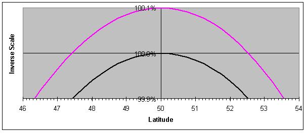
The black curve in this graph represents the percentage variation in distance on Earth compared to the map for the tangent specification. It shows that the design range of scale holds in the latitude range from 47.46°N to 52.49°N. In that range the scale is indeed within 0.1% of the designated scale. Note that all distances on the map correspond to a distance on the Earth of less than or equal to 5km. We have not used the allowed range of scale above 100%, and this is unnecessarily restrictive. We could map a greater latitude range within our design limits of scale if we made use of the other half of the allowed scale range.
To this end, suppose we specify a “secant” projection of 1:500,000 at the reference latitudes 47.46°N and 52.49°N. The red curve in the graph shows the resulting percentage variation in scale. The projection cone is still the same, tangent at 50°N, but the map now covers an extended latitude range, (from 46.36°N to 53.54°N), at the nominal scale of 1:500000, to within the specified accuracy.
The “secant” specification provides the map’s user with the information that, if he uses a 1:500000 scale to draw a track on the map, his measurements will slightly underrepresent distances on the earth in the latitude band between the reference latitudes, and slightly over-represent the distances on the earth when outside this band, but throughout the band and outside the band for an interval of about 20% the separation between the reference latitudes, the differences will be acceptable. Thus, the distance between the reference latitudes provides the user information that cannot be provided by simply a tangent specification.
In summary, the secant specification allows the cartographer more space to map to his intended scale, and provides the user information as to the precision in the area covered by the cartographer. - Are you sure the Lambert cone doesn’t pass through the Earth at the reference latitudes?
I am very sure. Consider the chart above, giving the distribution of the scale with respect to latitude for cones tangent at 50°N. Similar charts can be produced for cones tangent at any latitude; each will pass from zero at the poles to a maximum at the tangent latitude. Pairs of reference latitudes corresponding to the cone are found by drawing a horizontal line and noting the two places where it cuts the curve.
Suppose that, for all of these pairs, if the cone passes through one latitude circle, it also passes through the other. At least for a spherical Earth, that would mean the cone would be tangent to a latitude circle precisely midway between the two reference latitudes, and that in turn would mean the graph above was symmetric about the latitude 50°N.
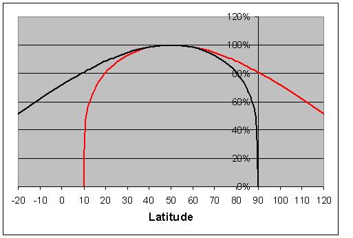
- Is it unreasonable to make a tangent specification with a secant specification whose latitudes are the same?
The Red curve in the above graph is the reflection of the inverse scale function (the black curve) in the 50°N latitude. Any spatial separation between the two, or any other distinctive differences, shows our supposition cannot be true, and Lambert projection cones do not generally pass through both reference latitudes.