

HYSPLIT models simulate the dispersion and trajectory of substances transported and dispersed through our atmosphere, over local to global scales.
HYSPLIT is a complete system for computing simple air parcel trajectories, as well as complex transport, dispersion, chemical transformation, and deposition simulations. HYSPLIT continues to be one of the most extensively used atmospheric transport and dispersion models in the atmospheric sciences community. A common application is a back trajectory analysis to determine the origin of air masses and establish source-receptor relationships. HYSPLIT has also been used in a variety of simulations describing the atmospheric transport, dispersion, and deposition of pollutants and hazardous materials. Some examples of the applications include tracking and forecasting the release of radioactive material, wildfire smoke, windblown dust, pollutants from various stationary and mobile emission sources, allergens and volcanic ash.
The model calculation method is a hybrid between the Lagrangian approach, using a moving frame of reference for the advection and diffusion calculations as the trajectories or air parcels move from their initial location, and the Eulerian methodology, which uses a fixed three-dimensional grid as a frame of reference to compute pollutant air concentrations (The model name, no longer meant as an acronym, originally reflected this hybrid computational approach). HYSPLIT has evolved over more than 30 years, from estimating simplified single trajectories based on radiosonde observations to a system accounting for multiple interacting pollutants transported, dispersed, and deposited over local to global scales.

Arial view of November 11, 2020 recycling plant fire in Houston, Texas. (Image courtesy of KHOU).
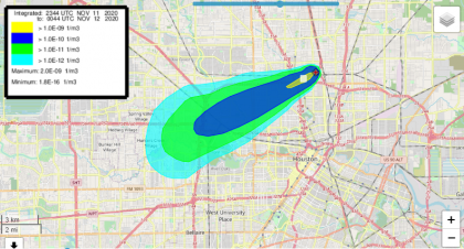
HYSPLIT Atmospheric Dispersion predictions from for Nov 11, 2020, northeast Houston area smoke plume. The WFO provided these information to the Houston Office of Emergency Management to inform the public alerts and response options.
The dispersion of a pollutant is calculated by assuming either puff or particle dispersion. In the puff model, puffs expand until they exceed the size of the meteorological grid cell (either horizontally or vertically) and then split into several new puffs, each with its share of the pollutant mass. In the particle model, a fixed number of particles are advected about the model domain by the mean wind field and spread by a turbulent component. The model’s default configuration assumes a 3-dimensional particle distribution (horizontal and vertical).
The model can be run interactively on the Web through the ARL READY system, or the code executable and meteorological data can be downloaded to a Windows or Mac PC. The web version has been configured with some limitations to avoid computational saturation of the ARL web server. The registered PC version is complete with no computational restrictions, except that users must obtain their own meteorological data files. The unregistered version is identical to the registered version except that plume concentrations cannot be calculated with forecast meteorology data files. The trajectory-only model has no restrictions, and forecast or archive trajectories may be computed with either version.
For more details, see the publication: NOAA’s HYSPLIT Atmospheric Transport and Dispersion Modeling System by Stein et al. in the December 2015 issue of the Bulletin of the American Meteorological Society. Citation: Stein, A. F., R. R. Draxler, G. D. Rolph, B. J. B. Stunder, M. D. Cohen, and F. Ngan. ” NOAA’s HYSPLIT Atmospheric Transport and Dispersion Modeling System”, Bulletin of the American Meteorological Society 96, 12 (2015): 2059-2077, accessed Oct 7, 2021, https://doi.org/10.1175/BAMS-D-14-00110.1
HYSPLIT Model Features
Trajectories
- Single or multiple (space or time) simultaneous trajectories
- Optional grid of initial starting locations
- Computations forward or backward in time
- Default vertical motion using omega field
- Other motion options: isentropic, isosigma, isobaric, isopycnic
- Trajectory ensemble option using meteorological variations
- Output of meteorological variables along a trajectory
- Integrated trajectory clustering option
Air Concentrations
- 3D particle dispersion or splitting puffs (top-hat or Gaussian)
- Instantaneous or continuous emissions, point or area sources
- Multiple resolution concentration output grids
- Fixed concentration grid or dynamic sampling
- Wet and dry deposition, radioactive decay, and resuspension
- Emission of multiple simultaneous pollutant species
- Automated source-receptor matrix computation
- Ensemble dispersion based on variations in meteorology, turbulence, or physics
- Concentration probability output for multiple simulations
- Integrated dust-storm emission algorithm
- Define rate constants to convert one species to another
- Mass can be transferred to a Eulerian module for global-scale simulations
Meteorology
- Model can run with multiple nested input data grids
- Links to ARL and NWS meteorological data server
- Access to forecasts and archives including NCAR/NCEP reanalysis
- Additional software to convert MM5, RAMS, COAMPS, WRF, and other data
- Utility programs to display and manipulate meteorological data
Common Features
- Tcl/Tk GUI with integrated html compatible help
- Viewer to display TOMS aerosol index with model particle positions
- Model restart from particle position files for plume initialization
- Model graphics displayed as Postscript files
- Converters to many other formats: GIF, GrADS, ArcView, Vis5D