Multiple Trajectories

Multiple Trajectories
Previous	HOME	Next	HIGHLIGHTS Advanced trajectory menu Use of SETUP.CFG file Multiple trajectories Trajectory matrix

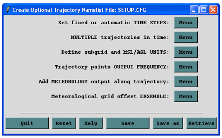
Normally trajectories are started only at the initial time at the locations/heights specified. Trajectories can also be started at regular time intervals from the same location by setting the restart interval to something other than 0. Clicking on the Advanced / Configuration Setup / Trajectory menu tab produces another menu (right) for entries in the optional trajectory namelist file.

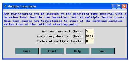
Clicking on Multiple trajectories in time menu button produces the menu shown to the right. To demonstrate the restart feature, change the restart interval to 3 hours, click Save, click Save again, and then and leave all the other trajectory parameters the same as in the original 700 hPa isobaric trajectory.

After clicking on Run Standard Model again a message box (shown at right) will appear to let you know that a SETUP.CFG configuration file exists and do you want to run with it. In this case since we want to run with the SETUP.CFG choose Run with SETUP.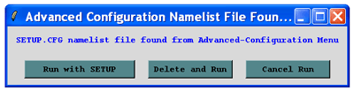

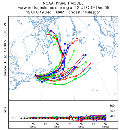
The resulting trajectory graphic shows new trajectories every 3 hours, terminating at the end of the 84 h computational period. Trajectories starting after the initial time will have a shorter duration. All trajectories can be set to have the same duration from the Advanced menu tab.

The GUI can only be used to configure up to 6 starting locations, however the model can support an unlimited number of locations. The GUI does have a shortcut method to configure a regular matrix of locations by defining three points, representing the lower left, upper right, and location increment from the starting location menu (see example to the right). Once configured, the Run Matrix option is selected through the Special Simulations menu tab of the Trajectory menu instead of Run Standard Model. This causes the locations defined by the grid (in this case 25) to be calculated and written to the CONTROL file.

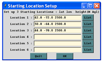
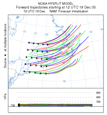
Trajectory Matrix Example

Rerun the 700 hPa isobaric case again but change the Total run time to 24 hours and choose the 3 source locations as shown to the right. Then from the Advanced / Configuration Setup / Trajectory menu choose the Define subgrid and MSL/AGL UNITS menu and set the height unit Relative to mean-sea-level because the terrain height varies across the matrix. Click Save and then set the restart interval back to 0 in the Multiple trajectories in time menu. Save this configuration and run the Matrix model from the Special Simulations menu. When finished set the Time Label Interval (hrs) to 0 in the Trajectory Display GUI) before executing the display (this makes a less cluttered display).

The resulting graphic should be similar to the graphic to the right showing the matrix of 24-h duration isobaric trajectories. Again there is very little differences noted between the trajectories indicating small temporal and spatial differences in the meteorology in this region. Note that we are using spatial and temporal offsets to ascertain the trajectory error or in this case sensitivity to the meteorological data.

HOME