Multiple Trajectories |
|||
 Previous |
 Next |
|
|
Multiple Trajectory Starting Locations
After choosing the meteorological data set, the first menu (below) gives the user the option of computing trajectories from 1, 2 or 3 different starting locations. Choosing more than one can be useful if more than one trajectory is needed to be plotted on the same map. The only limitation is that the starting heights (up to 3) must be the same for each location.

Trajectory Restart Option
| Normally trajectories are started only at the initial
time at the locations and heights specified by the user. However, by entering
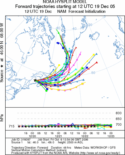
a value (hours) in the Start a new trajectory every field,
trajectories can be started at regular time intervals from the same location.
At this time, a maximum of 24 trajectories for a total of 48 hours duration are allowed
on HYSPLIT-WEB due to the resources needed to compute these trajectories. To demonstrate this feature see Example 4 Powerpoint (Ex4_hysplit.ppt)] or, change the restart interval to 3 and leave all the other parameters the same as in the original 700 hPa isobaric trajectory, i.e.,
|
|
Trajectory Matrix Option
 Although HYSPLIT-WEB can be used to configure only up to 3 starting
locations, the model can support an unlimited number of locations.
HYSPLIT-WEB and PC HYSPLIT have a shortcut method to configure a regular matrix
of locations by defining three points, representing the lower left,
upper right, and location increment. HYSPLIT-WEB does have a limitation of
125 starting locations which represents about a 11x11 lat/lon grid with a
1 degree horizontal spacing.
Trajectory Matrix Example
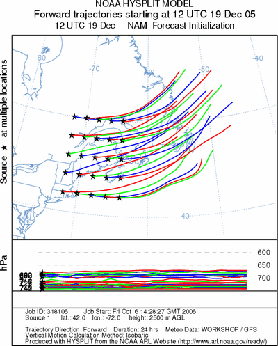
For this example see Example 5 Powerpoint (Ex5_hysplit.ppt)or,
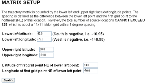
| After choosing a Matrix run and clicking
Next, a menu for entering the 3 matrix starting locations will
be presented (right). Other than entering 3 locations the rest of the
configuration is similar to a normal trajectory computation except that the locations
defined by the matrix grid will be calculated and written to the
CONTROL file before
executing the run. Rerun the 700 hPa isobaric case again but change the Total run
time to 24 hours and choose the 3 source locations as shown
to the right (42.0,-72.0), (50.0,-64.0) and
(44.0,-70.0). This configuration
will produce 25 starting locations separated by 2 degrees of latitude (~222 km). Also,
set the restart interval back to 0 if it is not 0. |
|
Trajectory Ensemble Option
 Frequently it is necessary to attribute a pollutant measurement to a specific source
location. One approach is to compute a backward trajectory to determine the air’s origin.
Although it is not uncommon to see sources identified by a single trajectory, the
uncertainties inherent in a single-trajectory can preempt its utility. One way to reduce
those uncertainties would be to compute multiple trajectories, in height, time, and space.
HYSPLIT can be configured to automatically run trajectories in an ensemble fashion from the
chosen starting location. Each member of the trajectory ensemble is calculated by
offsetting the meteorological data by a fixed grid factor (HYSPLIT-WEB assumes one
meteorological grid point in the horizontal and 0.01 sigma units in the vertical). This
results in 27 members for all-possible offsets in X,Y, and Z. Note: the starting height
should be greater than 250 m for optimal configuration of the ensemble.
Trajectory Ensemble Example
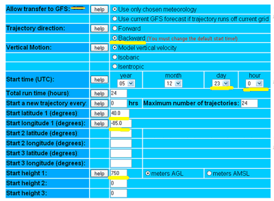
For this example see Example 6 Powerpoint (Ex6_hysplit.ppt)or,
For this example choose:
|
|
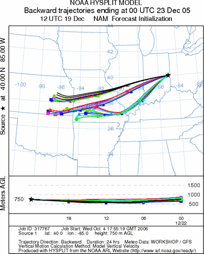 The resulting plot (right) shows that 3 different paths are possible depending
on the selected location in X, Y, and Z. This method gives the user a
sense of the sensitivity of the chosen starting location within the meteorological
grid as well as an "envelope" of the uncertainty about the single trajectory result.
 Previous |
 Next |
