Concentration Ensembles |
|||
 Previous |
 Next |
|
|
Instead of creating a single deterministic air concentration simulation, several programs are included with HYSPLIT that can be used to combine multiple HYSPLIT simulations into a single graphic that represents some variation of a concentration probability. The simplest approach is to run the model multiple times varying some parameter.
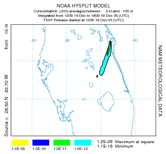
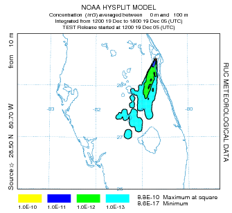
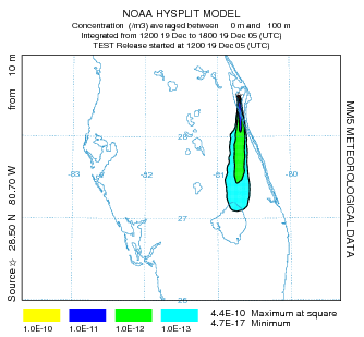
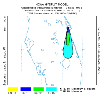
In the first case the model is run with multiple meteorological data (in the Advanced / Concentration Setup / Concentration, click on Reset and then Save). Each simulation was from 28.5N, 80.7W at 10 m. Also, to convert these data to a probability format below, the binary output files must be named with the suffix .001, .002, etc. in the Definition of Concentration Grid 1 menu. Be sure to Run with Setup. The 6 h average concentration graphic for each meteorological data set is given below for data from the NAM 12 km, the NAM 40 km, the RUC 20 km, the AFWAMM5 15 km, the AFWAMM5 45 km, and the GFS 1 degree. Notice that the NAM and RUC results show more of a westward component than the other 3 model results.
 |
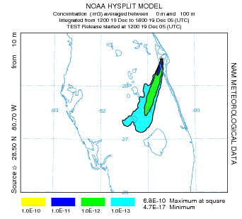 |
| NAM 12 km | NAM 40 km |
 |
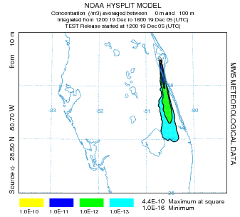 |
| RUC 20 km | AFWA MM5 15 km |
 |
 |
| AFWA MM5 45 km | GFS 1 Degree |
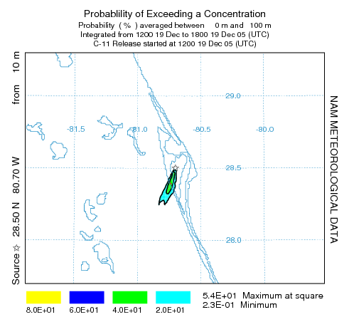
Now before running the ensemble display program the base name of the concentration files that were just created (cdump.001 to cdump.006) must be corrected in the Definition of Concentration Grid 1 menu. Change the last one selected, in this case cdump.006 to cdump (this is automatically taken care of by the GUI if running a one meteorological dataset internal ensemble as shown below). Save the setup, but do not rerun the model. This creates a new CONTROL file with the proper base name cdump. Now select Ensemble from the Concentration / Display Options menu. Three display options are available on this menu: the Number of Members, Mean, Variance, Probability of Concentration (probability of exceeding a given concentration), and the Concentration at Percentile (concentration at different probability levels).
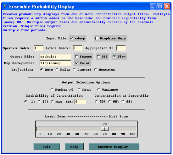
Selecting the Probability of Concentration at 1%, results in a probability plot at the 10-11 level.
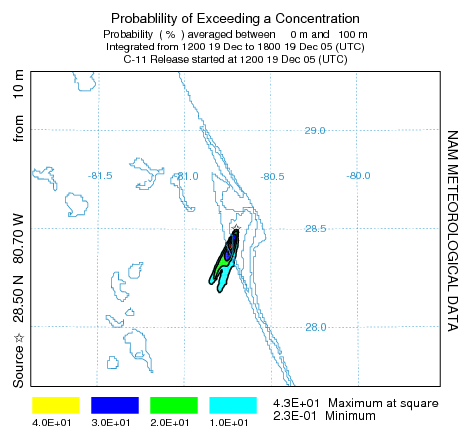
Another possibility is to generate an internal ensemble from a single meteorological data set. This computation is part of HYSPLIT and can be selected as the Run Ensemble option from the Concentration / Special Simulations menu tab. In these simulations the meteorological data are perturbed to test the sensitivity of the simulation to the flow field. The meteorological grid is offset in either X, Y, and Z for each member of the ensemble. The calculation offset for each member of the ensemble is determined by the grid factor and can be adjusted in the Advanced / Configuration Setup / Concentration menu. The default offset is one meteorological grid point in the horizontal and 0.01 sigma units in the vertical. The result is twenty-seven ensemble members for all offsets. Because the ensemble calculation offsets the starting point, it is suggested that for ground-level sources, the starting point height should be at least 0.01 sigma (about 250 m) above the ground. The ensemble for the NAM 40 km case is shown below (this may take several minutes to display).
 Previous |
 Next |